Tektronix TBS1000B and TBS1000B-EDU series digital storage oscilloscopes

Zoom function: Press [Zoom] to zoom in on specific parts of the waveform, supporting X1/X2/X5/X10 zoom ratios

3. Trigger Controls

Trigger type key parameters applicable scenarios

Edge triggered slope (rising/falling), coupling (AC/DC/noise suppression), stable display of conventional signals (sine wave/square wave)

Video trigger standards (NTSC/PAL/SECAM), synchronous (field/line) composite video signal testing, such as television signals

Pulse width triggering conditions (=≠<>), width (33ns-10s), polarity (positive/negative) capture abnormal pulses (such as spikes, narrow pulses)

Trigger mode:

Auto: Automatically scans without triggering, suitable for signal exploration

Normal: Only displayed when triggered, suitable for stable signal observation

Single: Single capture, suitable for transient signals (such as relay arcs)

4. Acquisition Controls

The working principle of the collection mode is applicable to different scenarios

Sampling mode equidistant sampling, 1 sampling point=1 waveform point for most conventional signals

Peak detection mode records the maximum/minimum values within each interval, captures narrow pulses (≥ 10ns), and reduces aliasing

After multiple acquisitions in average mode (4/16/64/128 times optional), suppress random noise and improve signal clarity

Measurement and analysis functions

1. Basic measurement techniques

Voltage measurement:

Peak to Peak Value (Vp-p): The difference between the maximum and minimum values of the signal, calculated by multiplying the number of vertical partitions by volts per grid and the probe attenuation ratio

Amplitude: Voltage from ground to signal peak, for example: 2V/div x 3 zones x 10X probe=60V

Time measurement:

Cycle/frequency: Cycle=number of horizontal partitions x seconds/grid, frequency=1/cycle

Pulse width: time interval at 50% amplitude, rise/fall time: time interval at 10% -90% amplitude

Phase difference measurement: Turn on XY mode and use the Lissajous diagram to determine (for example, when the frequency ratio is 1:1, the straight line is 0 ° and the circle is 90 °)

2. Automatic measurement and FFT analysis

Automatic measurement:

Supports 34 types, including time class (cycle, frequency, delay), amplitude class (peak to peak, overshoot), and count class (pulse number, edge number)

Up to 6 measurement results can be displayed simultaneously, with an update frequency of approximately 2 times per second

FFT analysis:

Window function selection: Hanning window (excellent frequency resolution), flat top window (excellent amplitude accuracy), rectangular window (transient analysis)

Nyquist frequency: half of the sampling rate. Exceeding this frequency will result in aliasing, which needs to be resolved by increasing the sampling rate or filtering

Spectrum measurement: supports cursor measurement of frequency (Hz) and amplitude (dB, 0dB=1VRMS)

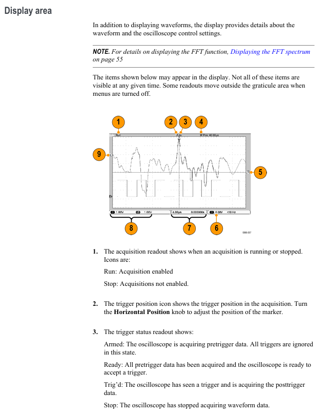
Data storage and transmission

1. USB flash drive operation

Storage content and capacity (approximately per 1MB):

250 setup files (. SET)

18 waveform files (. CSV, containing 2500 point time amplitude data)

16 image files (BMP/JPG)

Key operations:

Save: [Save/Recall] ->Select "Save Image/Set/Waveform" ->Automatic Naming (e.g. TEK0000. BMP)

Recall: [Save/Recall] → Select "Recall Setup/Waveform" → Select file

Format: [Utility] → [File Utilities] → [Format], note to delete all data

2. Connection between PC and GPIB

PC connection:

Install OpenChoice software (official website download)

Connect the USB cable between the oscilloscope's rear USB device port and the PC

Install the driver as prompted, supporting waveform transmission and remote control

GPIB connection:

Connect oscilloscope and GPIB controller through TEK-USB-488 adapter

[Utility] → [GPIB Setup] Set address (default 1)

Run GPIB software to achieve multi device collaborative control

Application Cases (Selected)

1. Video signal testing

Connect the probe to the video output and set the coupling to AC

【 Trigger Menu 】 → Select 'Video' → Set standard to NTSC

Select "All Fields" or "Line Number" synchronously, and press [Autoset]

Adjust the time base to 500ns/div and observe the video line signal (including color synchronization signal)

2. Differential signal analysis

CH1 is connected to the positive terminal of the differential signal, CH2 is connected to the negative terminal, and the probes are both set to 10X

【 Math 】 → Select "Ch1-Ch2" to display the differential waveform

【 Acquire 】 → Set to 'Peak Detect' to capture signal overshoot/noise

Read differential signal amplitude and rise time using automatic measurement function

3. Education version course application (exclusive to EDU version)

Create a course on PC (download specialized software) and save it as an. xpkg file

Insert the USB flash drive into the oscilloscope, go to 【 Utility 】 → 【 Update Course 】 → Load Course

Select the experiment according to 'Course' and view the steps and theories

After completing the experiment, the Data Collection saves the data and generates a report containing waveforms

Appendix and Maintenance

1. Performance parameters (key)

Vertical system: resolution 8-bit, DC gain accuracy ± 3% (10mV-5V/div), input impedance 1M Ω//20pF